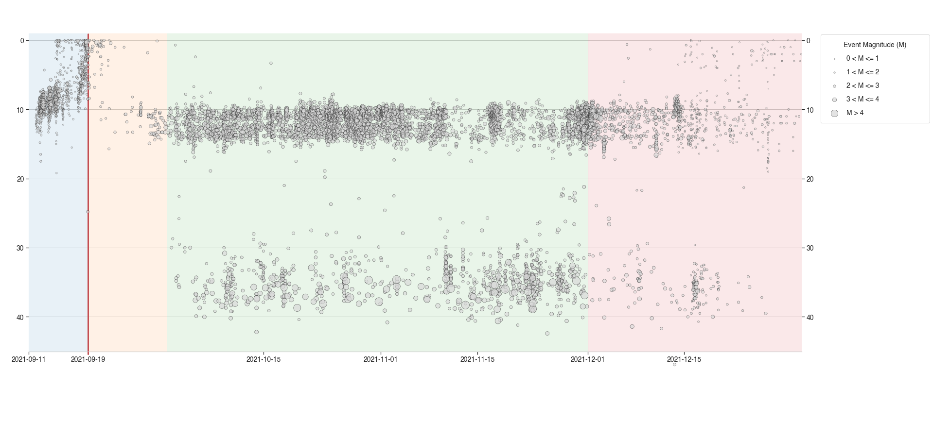
Main Timeline Figure
import pandas as pd
import matplotlib
import matplotlib.pyplot as plt
%matplotlib inline
import seaborn as sns
import numpy as np
sns.set_theme(style="whitegrid")
def make_category_columns(df):
df['Depth'] = 'Shallow (<18km)'
df.loc[(df['Depth(km)'] >= 18) & (df['Depth(km)'] <= 28), 'Depth'] = 'Interchange (18km>x>28km)'
df.loc[df['Depth(km)'] >= 28, 'Depth'] = 'Deep (>28km)'
df['Mag'] = 0
df.loc[(df['Magnitude'] >= 1) & (df['Magnitude'] <= 2), 'Mag'] = 1
df.loc[(df['Magnitude'] >= 2) & (df['Magnitude'] <= 3), 'Mag'] = 2
df.loc[(df['Magnitude'] >= 3) & (df['Magnitude'] <= 4), 'Mag'] = 3
df.loc[(df['Magnitude'] >= 4) & (df['Magnitude'] <= 5), 'Mag'] = 4
return dfVisualising Long term earthquake data
Data taken directly from the IGN Catalog
df_ign = pd.read_csv('./lapalma_ign.csv')
df_ign = make_category_columns(df_ign)
df_ign.head()
Loading...
df_ign['DateTime'] = pd.to_datetime(df_ign['DateTime'])
df_ign['DateTime']
0 2017-03-09 23:44:06
1 2017-03-10 00:16:10
2 2017-03-10 00:16:11
3 2017-03-10 03:20:26
4 2017-08-21 02:06:55
...
11342 2022-09-14 00:20:51
11343 2022-09-14 01:40:30
11344 2022-09-14 01:44:52
11345 2022-09-14 02:03:08
11346 2022-09-14 03:58:59
Name: DateTime, Length: 11347, dtype: datetime64[ns]df_ign_early = df_ign[df_ign['DateTime'] < '2021-09-11']
df_ign_pre = df_ign[(df_ign['DateTime'] >= '2021-09-11')&(df_ign['DateTime'] < '2021-09-19 14:13:00')]
df_ign_phase1 = df_ign[(df_ign['DateTime'] >= '2021-09-19 14:13:00')&(df_ign['DateTime'] < '2021-10-01')]
df_ign_phase2 = df_ign[(df_ign['DateTime'] >= '2021-10-01')&(df_ign['DateTime'] < '2021-12-01')]
df_ign_phase3 = df_ign[(df_ign['DateTime'] >= '2021-12-01')&(df_ign['DateTime'] <= '2021-12-31')]
df_erupt = df_ign[(df_ign['Date'] < '2022-01-01') & (df_ign['Date'] > '2021-09-11')]
df_erupt_1 = df_erupt[df_erupt['Magnitude'] < 1.0]
df_erupt_2 = df_erupt[(df_erupt['Magnitude'] >= 1.0)&(df_erupt['Magnitude'] < 2.0)]
df_erupt_3 = df_erupt[(df_erupt['Magnitude'] >= 2.0)&(df_erupt['Magnitude'] < 3.0)]
df_erupt_4 = df_erupt[(df_erupt['Magnitude'] >= 3.0)&(df_erupt['Magnitude'] < 4.0)]
df_erupt_5 = df_erupt[df_erupt['Magnitude'] > 4.0]
tab10_colors = (
    (0.12156862745098039, 0.4666666666666667,  0.7058823529411765  ),  # 1f77b4
    (1.0,                 0.4980392156862745,  0.054901960784313725),  # ff7f0e
    (0.17254901960784313, 0.6274509803921569,  0.17254901960784313 ),  # 2ca02c
    (0.8392156862745098,  0.15294117647058825, 0.1568627450980392  ),  # d62728
    (0.5803921568627451,  0.403921568627451,   0.7411764705882353  ),  # 9467bd
    (0.5490196078431373,  0.33725490196078434, 0.29411764705882354 ),  # 8c564b
    (0.8901960784313725,  0.4666666666666667,  0.7607843137254902  ),  # e377c2
    (0.4980392156862745,  0.4980392156862745,  0.4980392156862745  ),  # 7f7f7f
    (0.7372549019607844,  0.7411764705882353,  0.13333333333333333 ),  # bcbd22
    (0.09019607843137255, 0.7450980392156863,  0.8117647058823529),    # 17becf
)

tab20_colors = (
    (0.12156862745098039, 0.4666666666666667,  0.7058823529411765  ),  # 1f77b4
    (0.6823529411764706,  0.7803921568627451,  0.9098039215686274  ),  # aec7e8
    (1.0,                 0.4980392156862745,  0.054901960784313725),  # ff7f0e
    (1.0,                 0.7333333333333333,  0.47058823529411764 ),  # ffbb78
    (0.17254901960784313, 0.6274509803921569,  0.17254901960784313 ),  # 2ca02c
    (0.596078431372549,   0.8745098039215686,  0.5411764705882353  ),  # 98df8a
    (0.8392156862745098,  0.15294117647058825, 0.1568627450980392  ),  # d62728
    (1.0,                 0.596078431372549,   0.5882352941176471  ),  # ff9896
    (0.5803921568627451,  0.403921568627451,   0.7411764705882353  ),  # 9467bd
    (0.7725490196078432,  0.6901960784313725,  0.8352941176470589  ),  # c5b0d5
    (0.5490196078431373,  0.33725490196078434, 0.29411764705882354 ),  # 8c564b
    (0.7686274509803922,  0.611764705882353,   0.5803921568627451  ),  # c49c94
    (0.8901960784313725,  0.4666666666666667,  0.7607843137254902  ),  # e377c2
    (0.9686274509803922,  0.7137254901960784,  0.8235294117647058  ),  # f7b6d2
    (0.4980392156862745,  0.4980392156862745,  0.4980392156862745  ),  # 7f7f7f
    (0.7803921568627451,  0.7803921568627451,  0.7803921568627451  ),  # c7c7c7
    (0.7372549019607844,  0.7411764705882353,  0.13333333333333333 ),  # bcbd22
    (0.8588235294117647,  0.8588235294117647,  0.5529411764705883  ),  # dbdb8d
    (0.09019607843137255, 0.7450980392156863,  0.8117647058823529  ),  # 17becf
    (0.6196078431372549,  0.8549019607843137,  0.8980392156862745),    # 9edae5
)

tab20c_colors = (
    (0.19215686274509805, 0.5098039215686274,  0.7411764705882353  ),  # 3182bd
    (0.4196078431372549,  0.6823529411764706,  0.8392156862745098  ),  # 6baed6
    (0.6196078431372549,  0.792156862745098,   0.8823529411764706  ),  # 9ecae1
    (0.7764705882352941,  0.8588235294117647,  0.9372549019607843  ),  # c6dbef
    (0.9019607843137255,  0.3333333333333333,  0.050980392156862744),  # e6550d
    (0.9921568627450981,  0.5529411764705883,  0.23529411764705882 ),  # fd8d3c
    (0.9921568627450981,  0.6823529411764706,  0.4196078431372549  ),  # fdae6b
    (0.9921568627450981,  0.8156862745098039,  0.6352941176470588  ),  # fdd0a2
    (0.19215686274509805, 0.6392156862745098,  0.32941176470588235 ),  # 31a354
    (0.4549019607843137,  0.7686274509803922,  0.4627450980392157  ),  # 74c476
    (0.6313725490196078,  0.8509803921568627,  0.6078431372549019  ),  # a1d99b
    (0.7803921568627451,  0.9137254901960784,  0.7529411764705882  ),  # c7e9c0
    (0.4588235294117647,  0.4196078431372549,  0.6941176470588235  ),  # 756bb1
    (0.6196078431372549,  0.6039215686274509,  0.7843137254901961  ),  # 9e9ac8
    (0.7372549019607844,  0.7411764705882353,  0.8627450980392157  ),  # bcbddc
    (0.8549019607843137,  0.8549019607843137,  0.9215686274509803  ),  # dadaeb
    (0.38823529411764707, 0.38823529411764707, 0.38823529411764707 ),  # 636363
    (0.5882352941176471,  0.5882352941176471,  0.5882352941176471  ),  # 969696
    (0.7411764705882353,  0.7411764705882353,  0.7411764705882353  ),  # bdbdbd
    (0.8509803921568627,  0.8509803921568627,  0.8509803921568627  ),  # d9d9d9
)
from matplotlib.patches import Rectangle
import datetime as dt
from matplotlib.dates import date2num, num2date
matplotlib.rcParams['font.sans-serif'] = "Helvetica"
matplotlib.rcParams['font.family'] = "sans-serif"
matplotlib.rcParams['xtick.labelsize'] = 14
matplotlib.rcParams['ytick.labelsize'] = 14
matplotlib.rcParams['ytick.labelleft'] = True
matplotlib.rcParams['ytick.labelright'] = True
%matplotlib inline
fig = matplotlib.pyplot.figure(figsize=(24,12))
fig.tight_layout()
# Creating axis
# add_axes([xmin,ymin,dx,dy])
ax_min = fig.add_axes([0.01, 0.01, 0.01, 0.01])
ax_min.axis('off')
ax_max = fig.add_axes([0.99, 0.99, 0.01, 0.01])
ax_max.axis('off')
ax_timeline = fig.add_axes([0.04, 0.1, 0.92, 0.85])
ax_timeline.spines["top"].set_visible(False)
ax_timeline.spines["right"].set_visible(False)
ax_timeline.spines["left"].set_visible(False)
ax_timeline.grid(axis='x')
ax_timeline.axvline(x=dt.datetime(2021, 9, 19, 14, 13), ymin=0.075, ymax=0.972, color='r', linewidth=3)
def make_scatter(df, c, alpha=0.8):
M = 3*np.exp2(1.3*df['Magnitude'])
return ax_timeline.scatter(df['DateTime'], df['Depth(km)'], s=M, c=c, alpha=alpha, edgecolor='black', linewidth=0.5, zorder=2);
# make_scatter(df_erupt, c=tab20c_colors[-1])
points_1 = make_scatter(df_erupt_1, c=[tab20c_colors[-1]], alpha=0.5)
points_2 = make_scatter(df_erupt_2, c=[tab20c_colors[-1]], alpha=0.5)
points_3 = make_scatter(df_erupt_3, c=[tab20c_colors[-1]], alpha=0.6)
points_4 = make_scatter(df_erupt_4, c=[tab20c_colors[-1]], alpha=0.65)
points_5 = make_scatter(df_erupt_5, c=[tab20c_colors[-1]], alpha=0.7)
ax_timeline.tick_params(axis='x', labelrotation=0, bottom=True)
ax_timeline.set_ylabel('')
ax_timeline.yaxis.set_ticks_position('both')
ax_timeline.yaxis.set_ticks_position('both')
xticks = ax_timeline.get_xticks()
new_xticks = [date2num(pd.to_datetime('2021-09-11')),
date2num(pd.to_datetime('2021-09-19 14:13:00'))]
new_xticks = np.append(new_xticks, xticks[2:-1])
ax_timeline.set_xticks(new_xticks)
ax_timeline.invert_yaxis()
ax_timeline.spines['bottom'].set_position(('data', 45))
ax_timeline.margins(tight=True, x=0)
ax_timeline.legend(
[points_1, points_2, points_3, points_4, points_5],
['0 < M <= 1','1 < M <= 2','2 < M <= 3','3 < M <= 4','M > 4'],
loc='best', bbox_to_anchor=(1.02, 0.88, 0.15, 0.1), fancybox=True, borderpad=1.0, labelspacing=1, mode="expand", title="Event Magnitude (M)", fontsize=14, title_fontsize=14)
ax_timeline.add_patch(Rectangle((date2num(pd.to_datetime('2021-09-11')), -1), date2num(pd.to_datetime('2021-09-19 14:13:00'))-date2num(pd.to_datetime('2021-09-11')), 46, color=tab20_colors[0], zorder=1, alpha=0.1))
ax_timeline.add_patch(Rectangle((date2num(pd.to_datetime('2021-09-19 14:13:00')), -1), date2num(pd.to_datetime('2021-10-01'))-date2num(pd.to_datetime('2021-09-19 14:13:00')), 46, color=tab20_colors[2], zorder=1, alpha=0.1))
ax_timeline.add_patch(Rectangle((date2num(pd.to_datetime('2021-10-01')), -1), date2num(pd.to_datetime('2021-12-01'))-date2num(pd.to_datetime('2021-10-01')), 46, color=tab20_colors[4], zorder=1, alpha=0.1))
ax_timeline.add_patch(Rectangle((date2num(pd.to_datetime('2021-12-01')), -1), date2num(pd.to_datetime('2021-12-31'))-date2num(pd.to_datetime('2021-12-01'))+1, 46, color=tab20_colors[6], zorder=1, alpha=0.1));
plt.savefig('timeline_grey_with_panels.eps', format='eps')
The PostScript backend does not support transparency; partially transparent artists will be rendered opaque.
from matplotlib.patches import Rectangle
import datetime as dt
from matplotlib.dates import date2num, num2date
matplotlib.rcParams['font.sans-serif'] = "Helvetica"
matplotlib.rcParams['font.family'] = "sans-serif"
matplotlib.rcParams['xtick.labelsize'] = 14
matplotlib.rcParams['ytick.labelsize'] = 14
matplotlib.rcParams['ytick.labelleft'] = True
matplotlib.rcParams['ytick.labelright'] = True
%matplotlib inline
fig = matplotlib.pyplot.figure(figsize=(24,12))
fig.tight_layout()
# Creating axis
# add_axes([xmin,ymin,dx,dy])
ax_min = fig.add_axes([0.01, 0.01, 0.01, 0.01])
ax_min.axis('off')
ax_max = fig.add_axes([0.99, 0.99, 0.01, 0.01])
ax_max.axis('off')
ax_timeline = fig.add_axes([0.04, 0.1, 0.92, 0.85])
ax_timeline.spines["top"].set_visible(False)
ax_timeline.spines["right"].set_visible(False)
ax_timeline.spines["left"].set_visible(False)
ax_timeline.grid(axis='x')
ax_timeline.axvline(x=dt.datetime(2021, 9, 19, 14, 13), ymin=0.075, ymax=0.972, color='r', linewidth=3)
def make_scatter(df, c, alpha=0.8):
M = 3*np.exp2(1.3*df['Magnitude'])
return ax_timeline.scatter(df['DateTime'], df['Depth(km)'], s=M, c=c, alpha=alpha, edgecolor='black', linewidth=0.5, zorder=2);
# make_scatter(df_erupt, c=tab20c_colors[-1])
points_1 = make_scatter(df_erupt_1, c=[tab20_colors[12]], alpha=0.3)
points_2 = make_scatter(df_erupt_2, c=[tab20_colors[16]], alpha=0.4)
points_3 = make_scatter(df_erupt_3, c=[tab20_colors[4]], alpha=0.5)
points_4 = make_scatter(df_erupt_4, c=[tab20_colors[2]], alpha=0.6)
points_5 = make_scatter(df_erupt_5, c=[tab20_colors[6]], alpha=0.8)
ax_timeline.tick_params(axis='x', labelrotation=0, bottom=True)
ax_timeline.set_ylabel('')
ax_timeline.yaxis.set_ticks_position('both')
ax_timeline.yaxis.set_ticks_position('both')
xticks = ax_timeline.get_xticks()
new_xticks = [date2num(pd.to_datetime('2021-09-11')),
date2num(pd.to_datetime('2021-09-19 14:13:00'))]
new_xticks = np.append(new_xticks, xticks[2:-1])
ax_timeline.set_xticks(new_xticks)
ax_timeline.invert_yaxis()
ax_timeline.spines['bottom'].set_position(('data', 45))
ax_timeline.margins(tight=True, x=0)
ax_timeline.legend(
[points_1, points_2, points_3, points_4, points_5],
['0 < M <= 1','1 < M <= 2','2 < M <= 3','3 < M <= 4','M > 4'],
loc='best', bbox_to_anchor=(1.02, 0.88, 0.15, 0.1), fancybox=True, borderpad=1.0, labelspacing=1, mode="expand", title="Event Magnitude (M)", fontsize=14, title_fontsize=14)
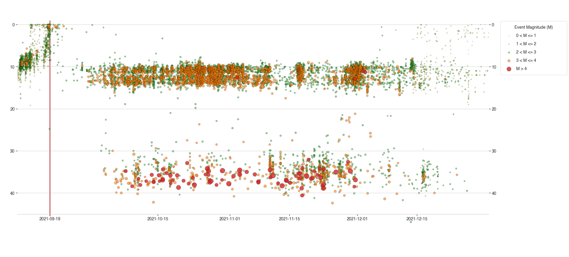
plt.savefig('timeline_colors.eps', format='eps')The PostScript backend does not support transparency; partially transparent artists will be rendered opaque.
from matplotlib.patches import Rectangle
import datetime as dt
from matplotlib.dates import date2num, num2date
matplotlib.rcParams['font.sans-serif'] = "Helvetica"
matplotlib.rcParams['font.family'] = "sans-serif"
matplotlib.rcParams['xtick.labelsize'] = 14
matplotlib.rcParams['ytick.labelsize'] = 14
matplotlib.rcParams['ytick.labelleft'] = True
matplotlib.rcParams['ytick.labelright'] = True
%matplotlib inline
fig = matplotlib.pyplot.figure(figsize=(24,12))
fig.tight_layout()
# Creating axis
# add_axes([xmin,ymin,dx,dy])
ax_min = fig.add_axes([0.01, 0.01, 0.01, 0.01])
ax_min.axis('off')
ax_max = fig.add_axes([0.99, 0.99, 0.01, 0.01])
ax_max.axis('off')
ax_timeline = fig.add_axes([0.04, 0.1, 0.92, 0.85])
ax_timeline.spines["top"].set_visible(False)
ax_timeline.spines["right"].set_visible(False)
ax_timeline.spines["left"].set_visible(False)
ax_timeline.grid(axis='x')
ax_timeline.axvline(x=dt.datetime(2021, 9, 19, 14, 13), ymin=0.075, ymax=0.972, color='r', linewidth=3)
def make_scatter(df, c, alpha=0.8):
M = 3*np.exp2(1.3*df['Magnitude'])
return ax_timeline.scatter(df['DateTime'], df['Depth(km)'], s=M, c=c, alpha=alpha, edgecolor='black', linewidth=0.5, zorder=2);
# make_scatter(df_erupt, c=tab20c_colors[-1])
points_1 = make_scatter(df_erupt_1, c=[tab20_colors[12]], alpha=0.3)
points_2 = make_scatter(df_erupt_2, c=[tab20_colors[16]], alpha=0.4)
points_3 = make_scatter(df_erupt_3, c=[tab20_colors[4]], alpha=0.5)
points_4 = make_scatter(df_erupt_4, c=[tab20_colors[2]], alpha=0.6)
points_5 = make_scatter(df_erupt_5, c=[tab20_colors[6]], alpha=0.8)
ax_timeline.tick_params(axis='x', labelrotation=0, bottom=True)
ax_timeline.set_ylabel('')
ax_timeline.yaxis.set_ticks_position('both')
ax_timeline.yaxis.set_ticks_position('both')
xticks = ax_timeline.get_xticks()
new_xticks = [date2num(pd.to_datetime('2021-09-11')),
date2num(pd.to_datetime('2021-09-19 14:13:00'))]
new_xticks = np.append(new_xticks, xticks[2:-1])
ax_timeline.set_xticks(new_xticks)
ax_timeline.invert_yaxis()
ax_timeline.spines['bottom'].set_position(('data', 45))
ax_timeline.margins(tight=True, x=0)
ax_timeline.legend(
[points_1, points_2, points_3, points_4, points_5],
['0 < M <= 1','1 < M <= 2','2 < M <= 3','3 < M <= 4','M > 4'],
loc='best', bbox_to_anchor=(1.02, 0.88, 0.15, 0.1), fancybox=True, borderpad=1.0, labelspacing=1, mode="expand", title="Event Magnitude (M)", fontsize=14, title_fontsize=14)
ax_timeline.add_patch(Rectangle((date2num(pd.to_datetime('2021-09-11')), -1), date2num(pd.to_datetime('2021-09-19 14:13:00'))-date2num(pd.to_datetime('2021-09-11')), 46, color=tab20_colors[0], zorder=1, alpha=0.1))
ax_timeline.add_patch(Rectangle((date2num(pd.to_datetime('2021-09-19 14:13:00')), -1), date2num(pd.to_datetime('2021-10-01'))-date2num(pd.to_datetime('2021-09-19 14:13:00')), 46, color=tab20_colors[2], zorder=1, alpha=0.1))
ax_timeline.add_patch(Rectangle((date2num(pd.to_datetime('2021-10-01')), -1), date2num(pd.to_datetime('2021-12-01'))-date2num(pd.to_datetime('2021-10-01')), 46, color=tab20_colors[4], zorder=1, alpha=0.1))
ax_timeline.add_patch(Rectangle((date2num(pd.to_datetime('2021-12-01')), -1), date2num(pd.to_datetime('2021-12-31'))-date2num(pd.to_datetime('2021-12-01'))+1, 46, color=tab20_colors[6], zorder=1, alpha=0.1));
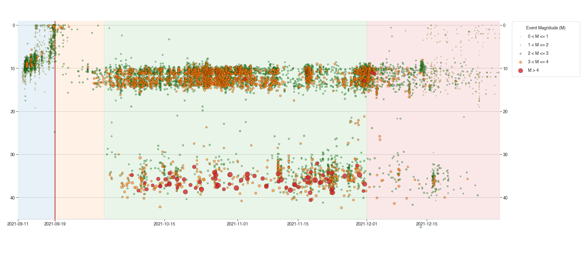
plt.savefig('timeline_colors_no_panels.eps', format='eps')The PostScript backend does not support transparency; partially transparent artists will be rendered opaque.
Cumulative Distrubtion Plots
def cumulative_events_mag_depth(df, hue='Depth', kind='scatter', ax=None, dpi=300, palette=None, kde=True):
matplotlib.rcParams['ytick.labelright'] = False
g = sns.jointplot(x="Magnitude", y="Depth(km)", data=df,
kind=kind, hue=hue, height=10, space=0.1, marginal_ticks=False, ratio=8, alpha=0.6,
hue_order=['Shallow (<18km)', 'Interchange (18km>x>28km)', 'Deep (>28km)'],
ax=ax, palette=palette, ylim=(-2,50), xlim=(0.3,5.6), edgecolor=".2", marginal_kws=dict(bins=20, hist_kws={'edgecolor': 'black'}))
if kde:
g.plot_joint(sns.kdeplot, color="b", zorder=1, levels=15, ax=ax)
g.fig.axes[0].invert_yaxis();
g.fig.set_dpi(dpi)
def cumulative_events_spatial(df, hue='Depth', kind='scatter', ax=None, dpi=300, palette=None):
g = sns.jointplot(x="Longitude", y="Depth(km)", data=df,
kind=kind, hue=hue, color="m", height=10, palette=palette,
hue_order=['Shallow (<18km)', 'Interchange (18km>x>28km)', 'Deep (>28km)', ], ax=ax, ylim=(-2,50))
g.plot_joint(sns.kdeplot, color="b", zorder=1, levels=15, ax=ax)
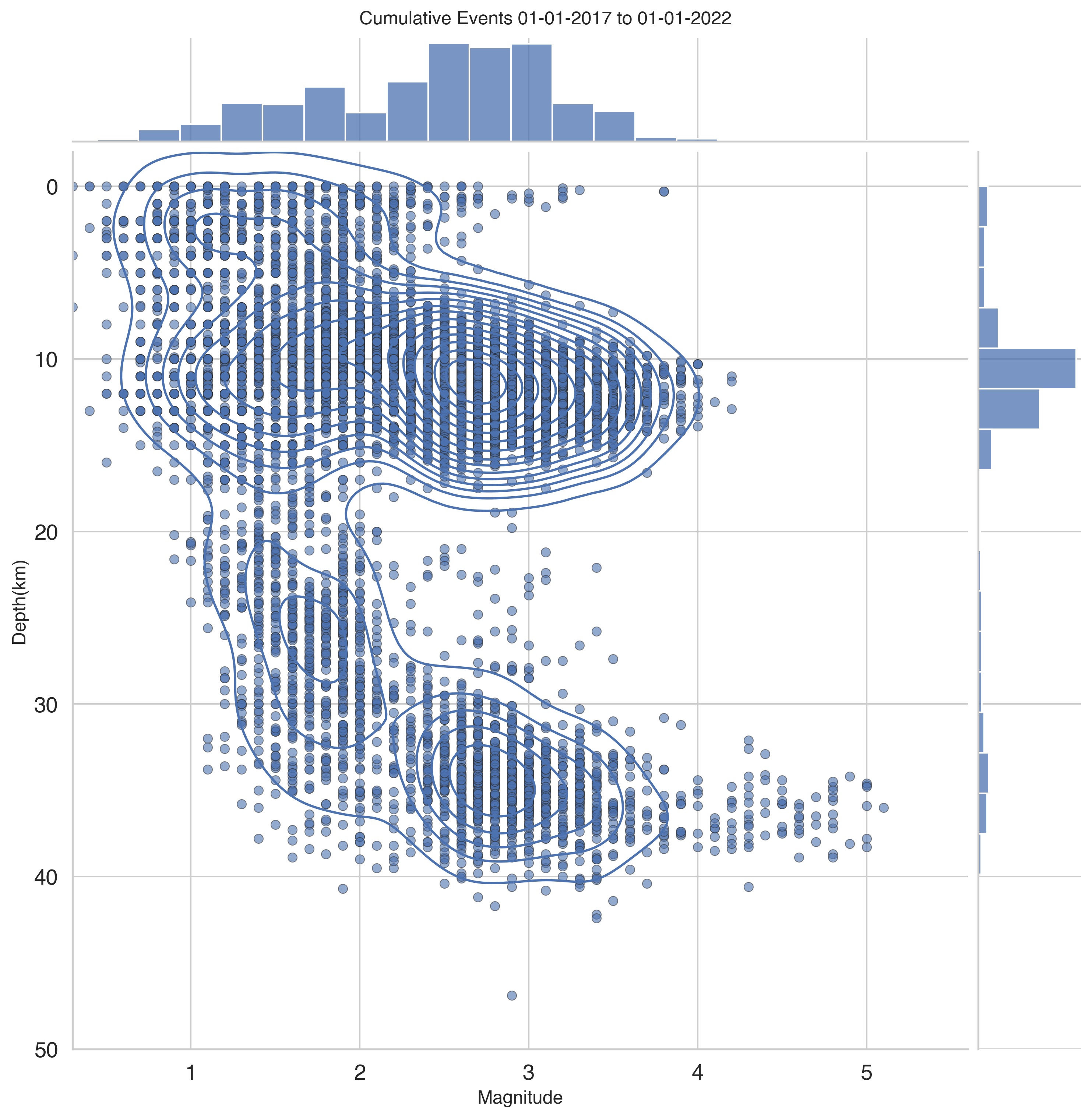
g.fig.axes[0].invert_yaxis();cumulative_events_mag_depth(df_ign, hue=None)
plt.suptitle('Cumulative Events 01-01-2017 to 01-01-2022', y=1.01);
plt.savefig('cuml_events_all.eps', format='eps')/opt/homebrew/Caskroom/miniforge/base/envs/lapalma-earthquakes/lib/python3.10/site-packages/seaborn/axisgrid.py:2203: UserWarning: The marginal plotting function has changed to `histplot`, which does not accept the following argument(s): hist_kws.
warnings.warn(msg, UserWarning)
The PostScript backend does not support transparency; partially transparent artists will be rendered opaque.
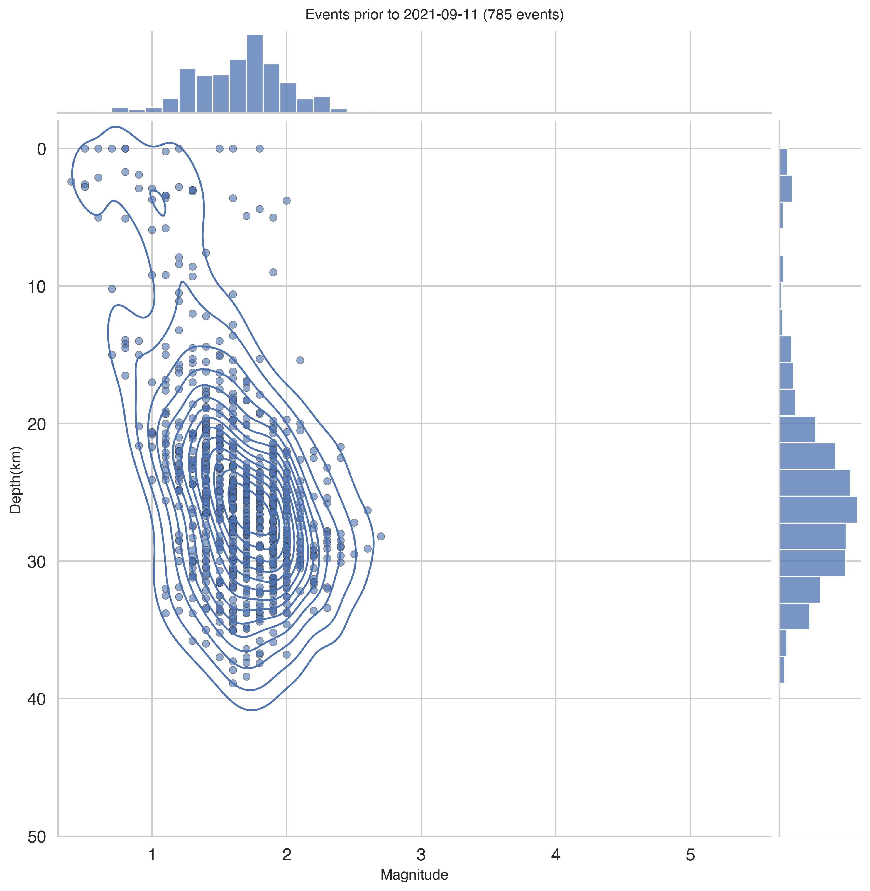
cumulative_events_mag_depth(df_ign_early, hue=None)
plt.suptitle(f'Events prior to 2021-09-11 ({len(df_ign_early.index)} events)', y=1.01)
plt.savefig('cuml_events_early.eps', format='eps')
/opt/homebrew/Caskroom/miniforge/base/envs/lapalma-earthquakes/lib/python3.10/site-packages/seaborn/axisgrid.py:2203: UserWarning: The marginal plotting function has changed to `histplot`, which does not accept the following argument(s): hist_kws.
warnings.warn(msg, UserWarning)
The PostScript backend does not support transparency; partially transparent artists will be rendered opaque.
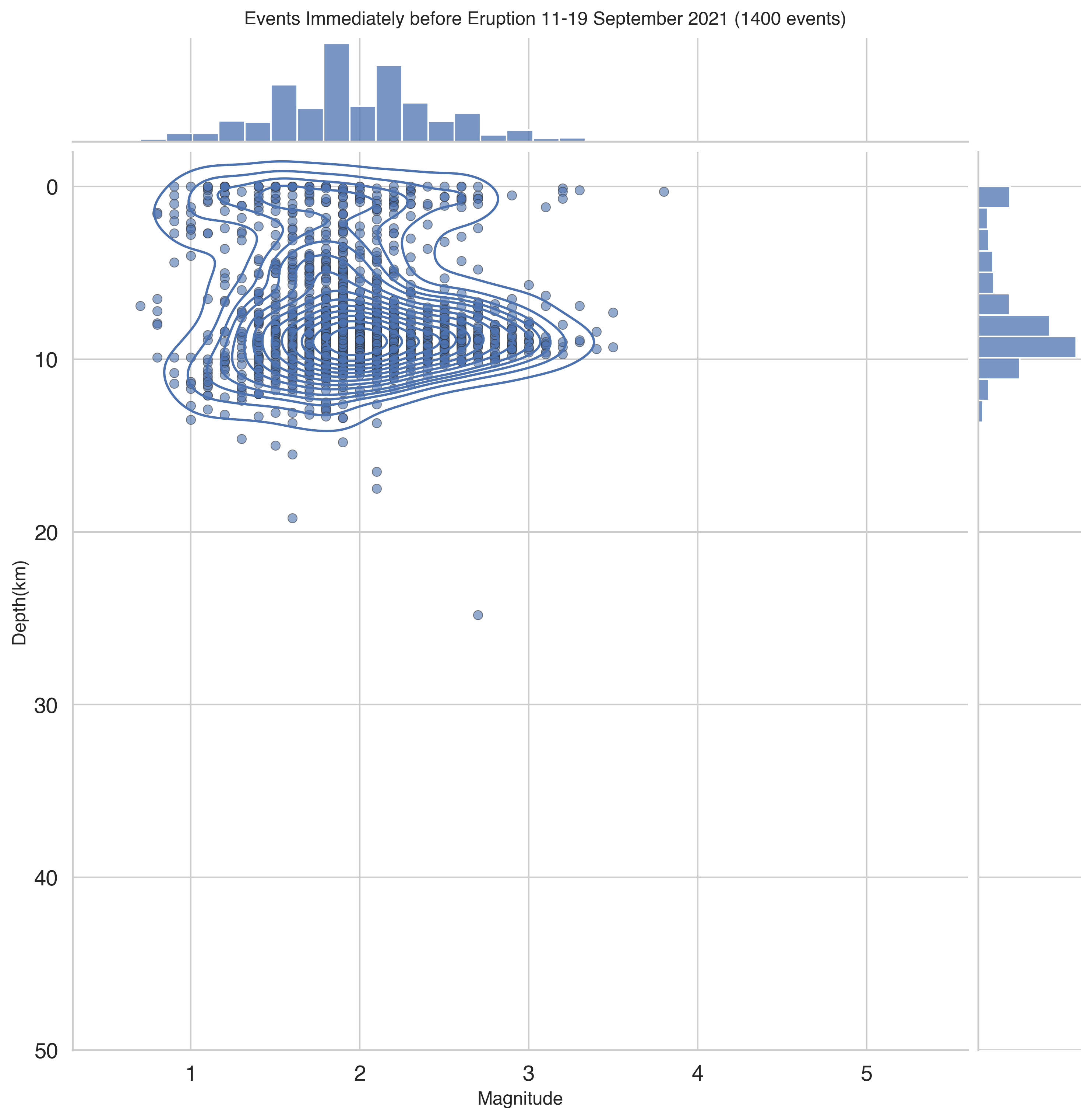
cumulative_events_mag_depth(df_ign_pre, hue=None)
plt.suptitle(f"Events Immediately before Eruption 11-19 September 2021 ({len(df_ign_pre.index)} events)", y=1.01);
plt.savefig('cuml_events_preerupt.eps', format='eps')
/opt/homebrew/Caskroom/miniforge/base/envs/lapalma-earthquakes/lib/python3.10/site-packages/seaborn/axisgrid.py:2203: UserWarning: The marginal plotting function has changed to `histplot`, which does not accept the following argument(s): hist_kws.
warnings.warn(msg, UserWarning)
The PostScript backend does not support transparency; partially transparent artists will be rendered opaque.
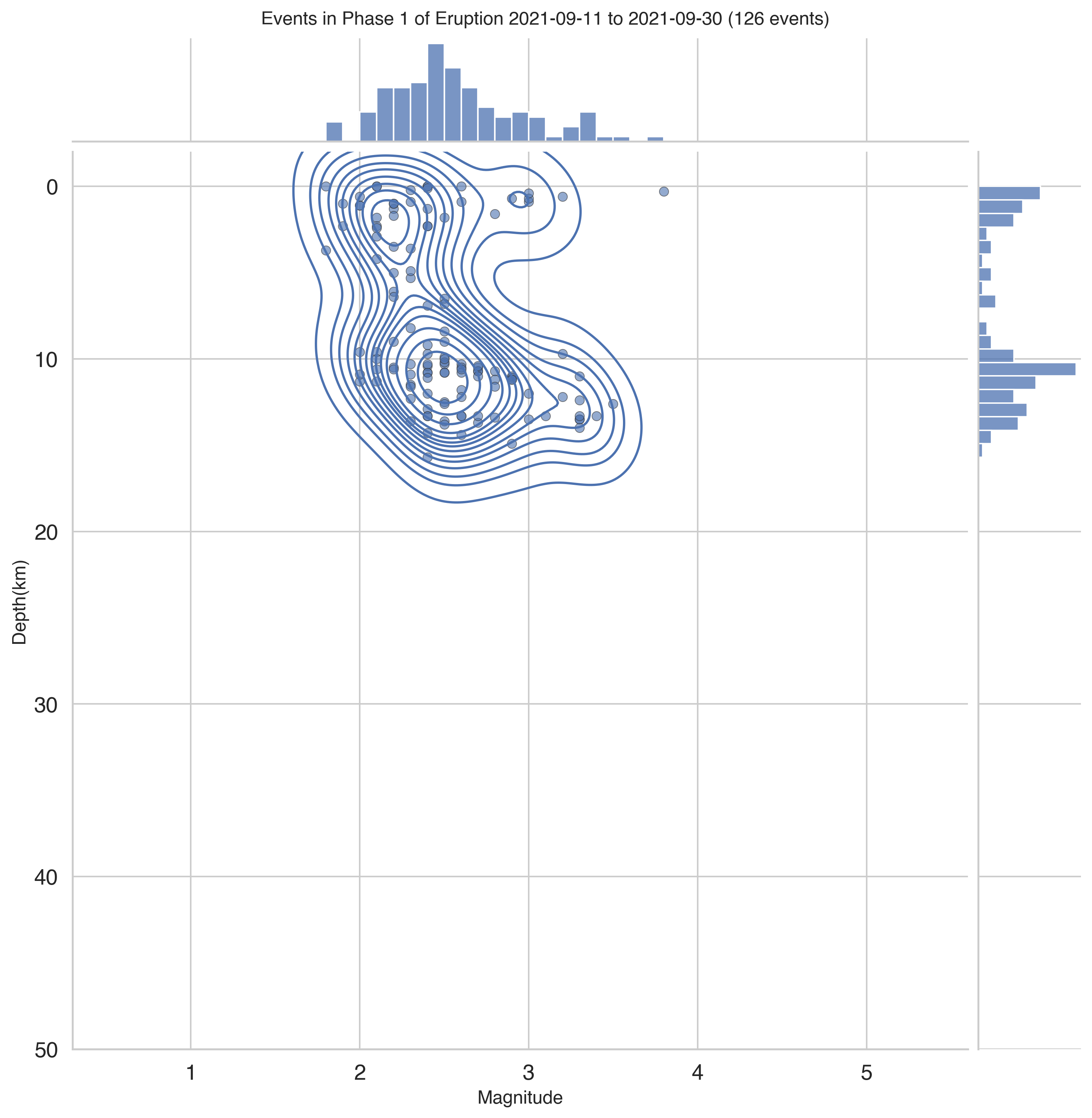
cumulative_events_mag_depth(df_ign_phase1, hue=None)
plt.suptitle(f"Events in Phase 1 of Eruption 2021-09-11 to 2021-09-30 ({len(df_ign_phase1.index)} events)", y=1.01);
plt.savefig('cuml_events_phase1.eps', format='eps')
/opt/homebrew/Caskroom/miniforge/base/envs/lapalma-earthquakes/lib/python3.10/site-packages/seaborn/axisgrid.py:2203: UserWarning: The marginal plotting function has changed to `histplot`, which does not accept the following argument(s): hist_kws.
warnings.warn(msg, UserWarning)
The PostScript backend does not support transparency; partially transparent artists will be rendered opaque.
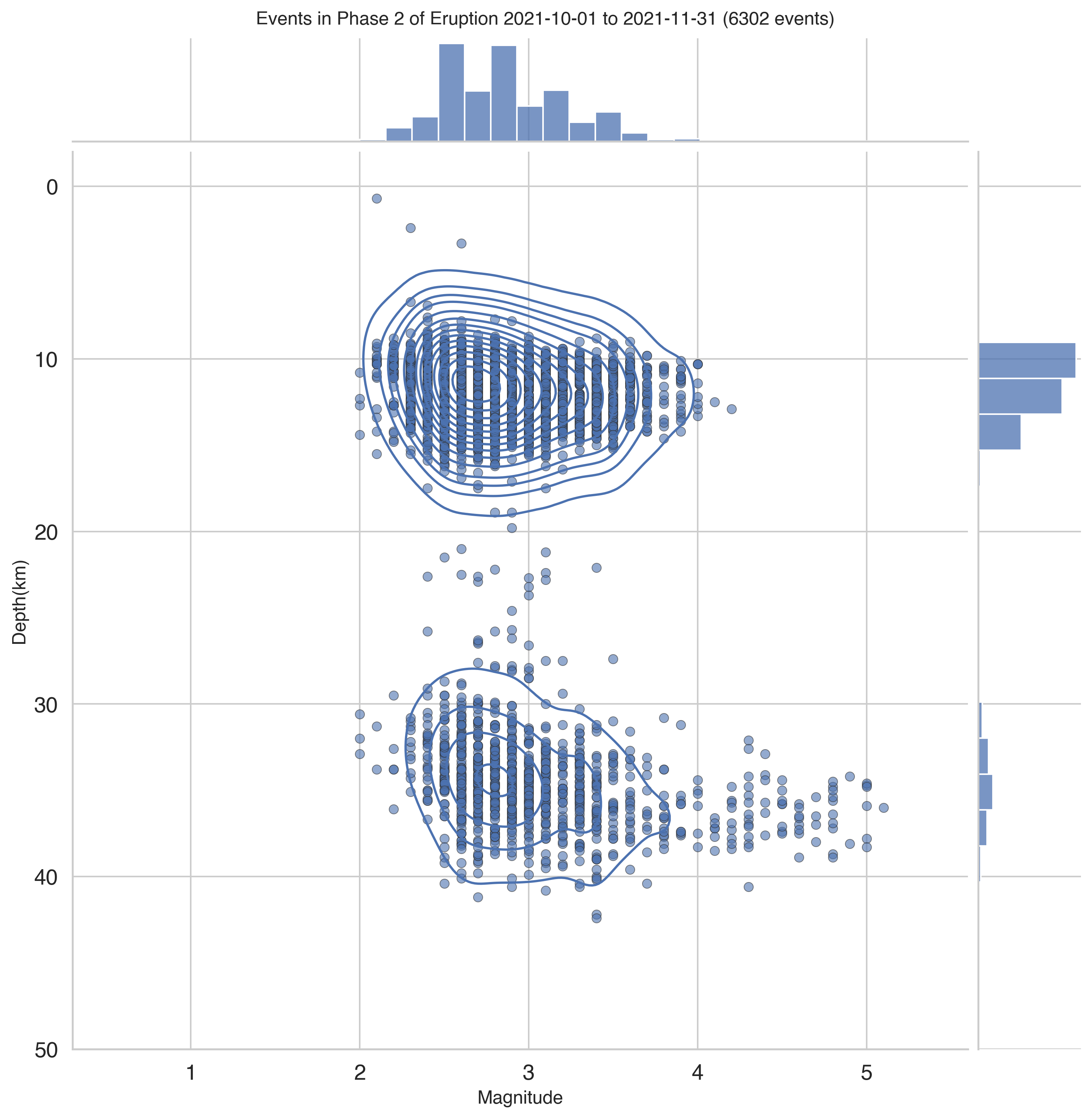
cumulative_events_mag_depth(df_ign_phase2, hue=None)
plt.suptitle(f"Events in Phase 2 of Eruption 2021-10-01 to 2021-11-31 ({len(df_ign_phase2.index)} events)", y=1.01);
plt.savefig('cuml_events_phase2.eps', format='eps')
/opt/homebrew/Caskroom/miniforge/base/envs/lapalma-earthquakes/lib/python3.10/site-packages/seaborn/axisgrid.py:2203: UserWarning: The marginal plotting function has changed to `histplot`, which does not accept the following argument(s): hist_kws.
warnings.warn(msg, UserWarning)
The PostScript backend does not support transparency; partially transparent artists will be rendered opaque.
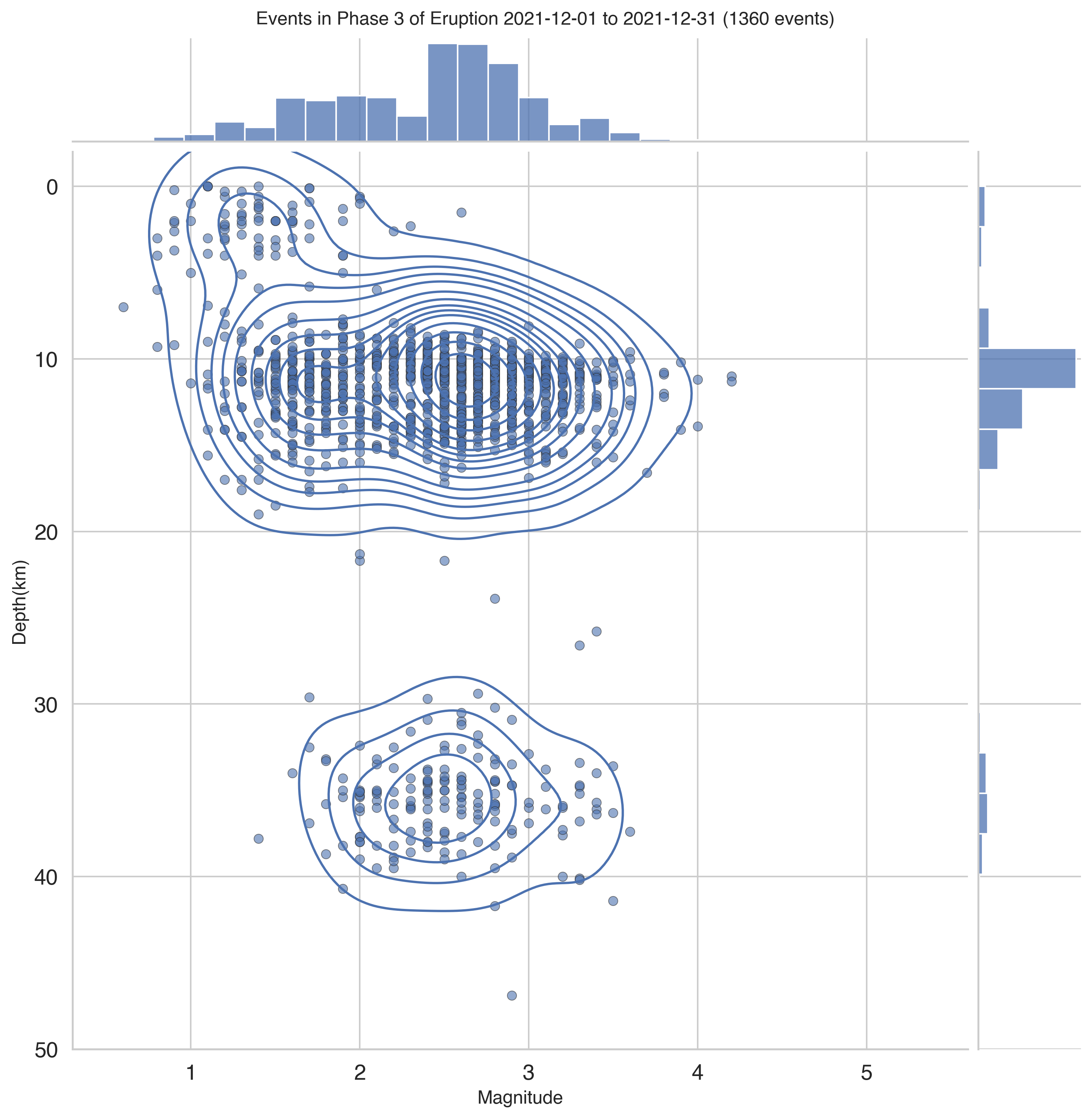
cumulative_events_mag_depth(df_ign_phase3, hue=None)
plt.suptitle(f"Events in Phase 3 of Eruption 2021-12-01 to 2021-12-31 ({len(df_ign_phase3.index)} events)", y=1.01);
plt.savefig('cuml_events_phase3.eps', format='eps')
/opt/homebrew/Caskroom/miniforge/base/envs/lapalma-earthquakes/lib/python3.10/site-packages/seaborn/axisgrid.py:2203: UserWarning: The marginal plotting function has changed to `histplot`, which does not accept the following argument(s): hist_kws.
warnings.warn(msg, UserWarning)
The PostScript backend does not support transparency; partially transparent artists will be rendered opaque.